Getting started
- Creating a starting population snapshot
- Running a simple neutral simulation
- Converting binary snapshots to text
Preparing files for simulation

Creating a starting population snapshot
Prior to running a simulation, the first thing you should do is create your own population snapshot. In SodaPop, a population is defined by a collection of cells, that are in turned defined by their genes. We will thus start by creating a gene file. A basic gene file looks like this:

It has a numeric identifier as well as an alphanumeric ID. The numeric identifier is important for the proper mapping of ancestral sequences. Genes are thus saved as [numericID].gene. You may keep an index of the alphanumeric ID corresponding to each gene file in the gene list (see below). Genes have an explicit nucleotide sequence and the corresponding translated amino acid sequence. The ‘E’ is a binary argument that denotes essentiality. The ‘DG’ is the Gibbs free energy (∆G, in kcal/mol), or stability of the protein. Finally, ‘CONC’ is the concentration (or abundance) of the gene.
To make a gene file, open a blank text file and make a tab-separated gene template with the fields above. Alternatively, you can open a preexisting gene file and copy its contents to a new file. Then you can change the values as you like. To create a gene file, retrieve the nucleotide and amino acid sequences of your gene of interest. The nucleotide sequence should have an exact 3 to 1 correspondence with the protein sequence. Furthermore, there should be no stop codons in the sequence. You can use the preexisting gene files as templates and overwrite the fields with your gene information.
The file gene_list.dat keeps an index of all the genes defined for the simulation. It lists the name of the gene files in your genes folder:
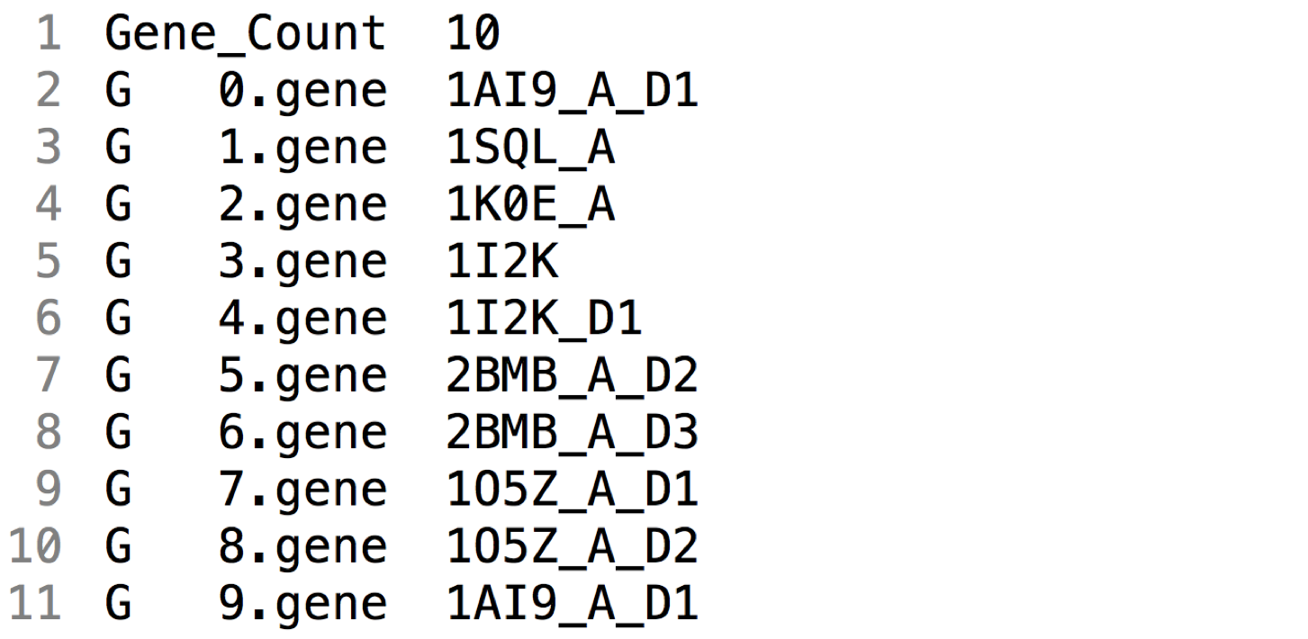
You can define as many genes and gene lists as you like. However, make sure you use the correct list when you run a simulation. If there is a mismatch between the genes of your intial population and the genes in your index list, the program will abort and issue an error.
Now that we’ve created our gene, we need to define a cell and its genome. Just like genes, cells also possess personal attributes such as a mutation rate. The file lists all the identifiers of genes in this cell, preceded by a ‘G’. Again, genes are indexed by their numeric identifier. The same goes for cells:

Once your cell is defined, you can create a population snapshot. The last layer in the hierarchy is the population description file. It lists the composition of the population we wish to create. In our case, we will start with a single lineage, but adding subpopulations is straightforward. The template below shows the information required to define a population. The count is the size of the population for that type of cell. The comment is optional and is ignored by the program.

To recapitulate, we must first create a gene file [1]. Then we define a cell file to include our gene(s) [2]. Finally, we create a population summary defining the initial clonal structure we want [3].
We can now build our starting population. We will use the program called sodasumm to build our population snapshot. If you run the program without any flag nor argument, it will display
sodasumm <population summary> [0-full | 1-single cell]
We need the population summary created above, and we must specify if we want to build the full population or strictly the first cell. The rationale behind this option is that as your population size increases to millions, populating the vector of cells gets computationally expensive. Extending the population with copies of a single cell is much faster than adding each cell one-by-one. However, you should only do this if your starting population is monoclonal. In any case, for smaller effective sizes, the cost of this operation is negligible.
Once you run sodasumm, a file called population.snap will appear in your working directory. This is your starting snapshot. You can move it to your start folder and rename it as you like. We advise to keep the .snap extension to distinguish between text and binary files.
Running a simple neutral simulation
Using our previously created population, we can run a very simple neutral simulation, that is, without selection. We can do this using the sample files packaged with the program. Try running the following command:
sodapop --sim-type stability –f 5 –p files/start/pop1K.snap –g files/genes/gene_list.dat –o neutral –n 1000 –m 1000 –t 10
The output should look like this:
Begin ...
Initializing matrix ...
Loading primordial genes file ...
Opening starting population snapshot ...
Creating directory out/neutral/snapshots ... OK
Constructing population from source files/start/pop1K.snap ...
Saving initial population snapshot ...
Starting evolution ...
Done.
Total number of mutation events: 10767
Let’s break down this command step by step:
sodapop is the main simulation utility (or program).
sim-type stability defines the type of input to be used for the simulation. In our case, we chose stability.
f 5 is the choice of fitness function. For more information on fitness functions, refer to the SodaPop manual (PDF). For now, just know that 5 is the mapping for the neutral fitness function.
p files/start/pop1K.snap is the argument for the starting population snapshot.
g files/genes/gene_list.dat is the argument for the gene index list.
o neutral is the prefix for output.
n 1000 is the population size.
m 1000 is the number of generations we would like to simulate.
t 10 is the interval at which the program saves a population snapshot.
Converting binary snapshots to text
To convert binary snapshots output by either of the programs above, you can use the program called sodasnap. Alternatively, adding the -a flag to your sodapop command will call analysis scripts once the simulation is done. This will automatically convert your snapshots to text, extract barcodes and plot general results. The following section discusses this in more detail.